deeplearning.ai homework:Class 2 Week 1 1.Initialization
Initialization
Welcome to the first assignment of “Improving Deep Neural Networks”.
Training your neural network requires specifying an initial value of the weights. A well chosen initialization method will help learning.
If you completed the previous course of this specialization, you probably followed our instructions for weight initialization, and it has worked out so far. But how do you choose the initialization for a new neural network? In this notebook, you will see how different initializations lead to different results.
A well chosen initialization can:
- Speed up the convergence of gradient descent
- Increase the odds of gradient descent converging to a lower training (and generalization) error
To get started, run the following cell to load the packages and the planar dataset you will try to classify.
1 | import numpy as np |
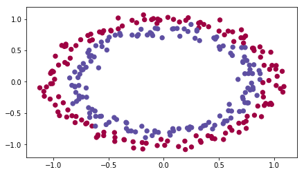
You would like a classifier to separate the blue dots from the red dots.
1 - Neural Network model
You will use a 3-layer neural network (already implemented for you). Here are the initialization methods you will experiment with:
- Zeros initialization – setting
initialization = "zeros"in the input argument. - Random initialization – setting
initialization = "random"in the input argument. This initializes the weights to large random values. - He initialization – setting
initialization = "he"in the input argument. This initializes the weights to random values scaled according to a paper by He et al., 2015.
Instructions: Please quickly read over the code below, and run it. In the next part you will implement the three initialization methods that this model() calls.
1 | def model(X, Y, learning_rate = 0.01, num_iterations = 15000, print_cost = True, initialization = "he"): |
2 - Zero initialization
There are two types of parameters to initialize in a neural network:
- the weight matrices
- the bias vectors
Exercise: Implement the following function to initialize all parameters to zeros. You’ll see later that this does not work well since it fails to “break symmetry”, but lets try it anyway and see what happens. Use np.zeros((…,…)) with the correct shapes.
1 | # GRADED FUNCTION: initialize_parameters_zeros |
1 | parameters = initialize_parameters_zeros([3,2,1]) |
W1 = [[ 0.  0.  0.]
 [ 0.  0.  0.]]
b1 = [[ 0.]
 [ 0.]]
W2 = [[ 0.  0.]]
b2 = [[ 0.]]
Expected Output:
| W1 | [[ 0. 0. 0.] [ 0. 0. 0.]] |
| b1 | [[ 0.] [ 0.]] |
| W2 | [[ 0. 0.]] |
| b2 | [[ 0.]] |
Run the following code to train your model on 15,000 iterations using zeros initialization.
1 | parameters = model(train_X, train_Y, initialization = "zeros") |
Cost after iteration 0: 0.6931471805599453
Cost after iteration 1000: 0.6931471805599453
Cost after iteration 2000: 0.6931471805599453
Cost after iteration 3000: 0.6931471805599453
Cost after iteration 4000: 0.6931471805599453
Cost after iteration 5000: 0.6931471805599453
Cost after iteration 6000: 0.6931471805599453
Cost after iteration 7000: 0.6931471805599453
Cost after iteration 8000: 0.6931471805599453
Cost after iteration 9000: 0.6931471805599453
Cost after iteration 10000: 0.6931471805599455
Cost after iteration 11000: 0.6931471805599453
Cost after iteration 12000: 0.6931471805599453
Cost after iteration 13000: 0.6931471805599453
Cost after iteration 14000: 0.6931471805599453
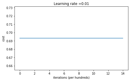
On the train set:
Accuracy: 0.5
On the test set:
Accuracy: 0.5
The performance is really bad, and the cost does not really decrease, and the algorithm performs no better than random guessing. Why? Lets look at the details of the predictions and the decision boundary:
1 | print ("predictions_train = " + str(predictions_train)) |
predictions_train = [[0 0 0 0 0 0 0 0 0 0 0 0 0 0 0 0 0 0 0 0 0 0 0 0 0 0 0 0 0 0 0 0 0 0 0 0 0
  0 0 0 0 0 0 0 0 0 0 0 0 0 0 0 0 0 0 0 0 0 0 0 0 0 0 0 0 0 0 0 0 0 0 0 0 0
  0 0 0 0 0 0 0 0 0 0 0 0 0 0 0 0 0 0 0 0 0 0 0 0 0 0 0 0 0 0 0 0 0 0 0 0 0
  0 0 0 0 0 0 0 0 0 0 0 0 0 0 0 0 0 0 0 0 0 0 0 0 0 0 0 0 0 0 0 0 0 0 0 0 0
  0 0 0 0 0 0 0 0 0 0 0 0 0 0 0 0 0 0 0 0 0 0 0 0 0 0 0 0 0 0 0 0 0 0 0 0 0
  0 0 0 0 0 0 0 0 0 0 0 0 0 0 0 0 0 0 0 0 0 0 0 0 0 0 0 0 0 0 0 0 0 0 0 0 0
  0 0 0 0 0 0 0 0 0 0 0 0 0 0 0 0 0 0 0 0 0 0 0 0 0 0 0 0 0 0 0 0 0 0 0 0 0
  0 0 0 0 0 0 0 0 0 0 0 0 0 0 0 0 0 0 0 0 0 0 0 0 0 0 0 0 0 0 0 0 0 0 0 0 0
  0 0 0 0]]
predictions_test = [[0 0 0 0 0 0 0 0 0 0 0 0 0 0 0 0 0 0 0 0 0 0 0 0 0 0 0 0 0 0 0 0 0 0 0 0 0
  0 0 0 0 0 0 0 0 0 0 0 0 0 0 0 0 0 0 0 0 0 0 0 0 0 0 0 0 0 0 0 0 0 0 0 0 0
  0 0 0 0 0 0 0 0 0 0 0 0 0 0 0 0 0 0 0 0 0 0 0 0 0 0]]
1 | plt.title("Model with Zeros initialization") |
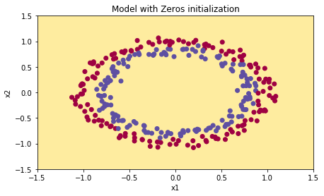
The model is predicting 0 for every example.
In general, initializing all the weights to zero results in the network failing to break symmetry. This means that every neuron in each layer will learn the same thing, and you might as well be training a neural network with for every layer, and the network is no more powerful than a linear classifier such as logistic regression.
What you should remember:
- The weights should be initialized randomly to break symmetry.
- It is however okay to initialize the biases to zeros. Symmetry is still broken so long as is initialized randomly.
3 - Random initialization
To break symmetry, lets intialize the weights randomly. Following random initialization, each neuron can then proceed to learn a different function of its inputs. In this exercise, you will see what happens if the weights are intialized randomly, but to very large values.
Exercise: Implement the following function to initialize your weights to large random values (scaled by *10) and your biases to zeros. Use np.random.randn(..,..) * 10 for weights and np.zeros((.., ..)) for biases. We are using a fixed np.random.seed(..) to make sure your “random” weights match ours, so don’t worry if running several times your code gives you always the same initial values for the parameters.
1 | # GRADED FUNCTION: initialize_parameters_random |
1 | parameters = initialize_parameters_random([3, 2, 1]) |
W1 = [[ 17.88628473   4.36509851   0.96497468]
 [-18.63492703  -2.77388203  -3.54758979]]
b1 = [[ 0.]
 [ 0.]]
W2 = [[-0.82741481 -6.27000677]]
b2 = [[ 0.]]
Expected Output:
| W1 | [[ 17.88628473 4.36509851 0.96497468] [-18.63492703 -2.77388203 -3.54758979]] |
| b1 | [[ 0.] [ 0.]] |
| W2 | [[-0.82741481 -6.27000677]] |
| b2 | [[ 0.]] |
Run the following code to train your model on 15,000 iterations using random initialization.
1 | parameters = model(train_X, train_Y, initialization = "random") |
Cost after iteration 0: inf
Cost after iteration 1000: 0.6231412804228252
Cost after iteration 2000: 0.5979042996377857
Cost after iteration 3000: 0.5636379908147912
Cost after iteration 4000: 0.5501412324370814
Cost after iteration 5000: 0.5444383478011093
Cost after iteration 6000: 0.5374380799952517
Cost after iteration 7000: 0.47560831443144236
Cost after iteration 8000: 0.39780215233411886
Cost after iteration 9000: 0.39347201638372875
Cost after iteration 10000: 0.3920273055562081
Cost after iteration 11000: 0.3892727039688806
Cost after iteration 12000: 0.386161047977093
Cost after iteration 13000: 0.3849881861838211
Cost after iteration 14000: 0.3827918021864143
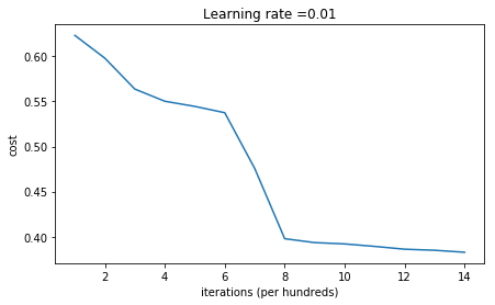
On the train set:
Accuracy: 0.83
On the test set:
Accuracy: 0.86
If you see “inf” as the cost after the iteration 0, this is because of numerical roundoff; a more numerically sophisticated implementation would fix this. But this isn’t worth worrying about for our purposes.
Anyway, it looks like you have broken symmetry, and this gives better results. than before. The model is no longer outputting all 0s.
1 | print (predictions_train) |
[[1 0 1 1 0 0 1 1 1 1 1 0 1 0 0 1 0 1 1 0 0 0 1 0 1 1 1 1 1 1 0 1 1 0 0 1 1
  1 1 1 1 1 1 0 1 1 1 1 0 1 0 1 1 1 1 0 0 1 1 1 1 0 1 1 0 1 0 1 1 1 1 0 0 0
  0 0 1 0 1 0 1 1 1 0 0 1 1 1 1 1 1 0 0 1 1 1 0 1 1 0 1 0 1 1 0 1 1 0 1 0 1
  1 0 0 1 0 0 1 1 0 1 1 1 0 1 0 0 1 0 1 1 1 1 1 1 1 0 1 1 0 0 1 1 0 0 0 1 0
  1 0 1 0 1 1 1 0 0 1 1 1 1 0 1 1 0 1 0 1 1 0 1 0 1 1 1 1 0 1 1 1 1 0 1 0 1
  0 1 1 1 1 0 1 1 0 1 1 0 1 1 0 1 0 1 1 1 0 1 1 1 0 1 0 1 0 0 1 0 1 1 0 1 1
  0 1 1 0 1 1 1 0 1 1 1 1 0 1 0 0 1 1 0 1 1 1 0 0 0 1 1 0 1 1 1 1 0 1 1 0 1
  1 1 0 0 1 0 0 0 1 0 0 0 1 1 1 1 0 0 0 0 1 1 1 1 0 0 1 1 1 1 1 1 1 0 0 0 1
  1 1 1 0]]
[[1 1 1 1 0 1 0 1 1 0 1 1 1 0 0 0 0 1 0 1 0 0 1 0 1 0 1 1 1 1 1 0 0 0 0 1 0
  1 1 0 0 1 1 1 1 1 0 1 1 1 0 1 0 1 1 0 1 0 1 0 1 1 1 1 1 1 1 1 1 0 1 0 1 1
  1 1 1 0 1 0 0 1 0 0 0 1 1 0 1 1 0 0 0 1 1 0 1 1 0 0]]
1 | plt.title("Model with large random initialization") |
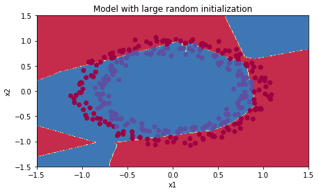
Observations:
- The cost starts very high. This is because with large random-valued weights, the last activation (sigmoid) outputs results that are very close to 0 or 1 for some examples, and when it gets that example wrong it incurs a very high loss for that example. Indeed, when , the loss goes to infinity.
- Poor initialization can lead to vanishing/exploding gradients, which also slows down the optimization algorithm.
- If you train this network longer you will see better results, but initializing with overly large random numbers slows down the optimization.
In summary:
- Initializing weights to very large random values does not work well.
- Hopefully intializing with small random values does better. The important question is: how small should be these random values be? Lets find out in the next part!
4 - He initialization
Finally, try “He Initialization”; this is named for the first author of He et al., 2015. (If you have heard of “Xavier initialization”, this is similar except Xavier initialization uses a scaling factor for the weights of sqrt(1./layers_dims[l-1]) where He initialization would use sqrt(2./layers_dims[l-1]).)
Exercise: Implement the following function to initialize your parameters with He initialization.
Hint: This function is similar to the previous initialize_parameters_random(...). The only difference is that instead of multiplying np.random.randn(..,..) by 10, you will multiply it by , which is what He initialization recommends for layers with a ReLU activation.
1 | # GRADED FUNCTION: initialize_parameters_he |
1 | parameters = initialize_parameters_he([2, 4, 1]) |
W1 = [[ 1.78862847  0.43650985]
 [ 0.09649747 -1.8634927 ]
 [-0.2773882  -0.35475898]
 [-0.08274148 -0.62700068]]
b1 = [[ 0.]
 [ 0.]
 [ 0.]
 [ 0.]]
W2 = [[-0.03098412 -0.33744411 -0.92904268  0.62552248]]
b2 = [[ 0.]]
Expected Output:
| W1 | [[ 1.78862847 0.43650985] [ 0.09649747 -1.8634927 ] [-0.2773882 -0.35475898] [-0.08274148 -0.62700068]] |
| b1 | [[ 0.] [ 0.] [ 0.] [ 0.]] |
| W2 | [[-0.03098412 -0.33744411 -0.92904268 0.62552248]] |
| b2 | [[ 0.]] |
Run the following code to train your model on 15,000 iterations using He initialization.
1 | parameters = model(train_X, train_Y, initialization = "he") |
Cost after iteration 0: 0.8830537463419761
Cost after iteration 1000: 0.6879825919728063
Cost after iteration 2000: 0.6751286264523371
Cost after iteration 3000: 0.6526117768893807
Cost after iteration 4000: 0.6082958970572938
Cost after iteration 5000: 0.5304944491717495
Cost after iteration 6000: 0.4138645817071794
Cost after iteration 7000: 0.3117803464844441
Cost after iteration 8000: 0.23696215330322562
Cost after iteration 9000: 0.18597287209206836
Cost after iteration 10000: 0.1501555628037181
Cost after iteration 11000: 0.12325079292273544
Cost after iteration 12000: 0.09917746546525937
Cost after iteration 13000: 0.08457055954024276
Cost after iteration 14000: 0.07357895962677366
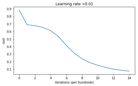
On the train set:
Accuracy: 0.993333333333
On the test set:
Accuracy: 0.96
1 | plt.title("Model with He initialization") |
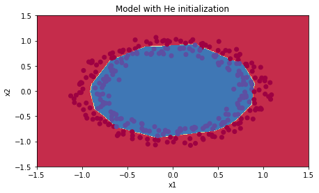
Observations:
- The model with He initialization separates the blue and the red dots very well in a small number of iterations.
5 - Conclusions
You have seen three different types of initializations. For the same number of iterations and same hyperparameters the comparison is:
| Model | Train accuracy | Problem/Comment |
What you should remember from this notebook:
- Different initializations lead to different results
- Random initialization is used to break symmetry and make sure different hidden units can learn different things
- Don’t intialize to values that are too large
- He initialization works well for networks with ReLU activations.
